I’ve started to train for a half marathon, just finishing week 5 of the 12 week Nike+ running coach half marathon program. I just want to know- how quickly can I expect to improve my running pace? I’m NOT a runner, and I’m very slow. By “not a runner”, I mean I had never run more than 4 miles at once before this program and not a single mile at all in the last two years. By “slow”, I mean that I am a 5’2″ girl who has a hard time keeping up with people I walk next to. To clarify further, because I recently read a comment somewhere on the interwebs about someone who was “slow” with a “sluggish pace” of 9’45” (HA, that’s my fastest mile!), I’ll just let you also know that my all time average pace with Nike+ Running app so far is 13’12”.
Anyway, I’ve spent a lot of time researching (read: googling constantly) how to go from basically no running to running a half marathon in just 12 weeks, and the interwebs have left me unsatisfied. I have zero desire to be a real distance runner (running a marathon sounds insane to me), and I have zero desire to be a fast runner and hate sprinting. I would just like to finish the half marathon in a time that is appropriate for my age/gender/capabilities.
The problem is that there is plenty of data about average half marathon finish times and paces for age/gender groups (see e.g., http://www.pace-calculator.com/average-half-marathon-pace-by-age-sex.php, 10’44” for 30 yo women?? hmmm, a 2:20 finish time seems too fast for me), but who cares if this says nothing about your actual capabilities!?!? Half marathons are full of runners!! What about me?? All of these crazy running addicts are skewing the data for us normies, and I’m not taking the advice that my goal should be to “finish.” That’s nice, but clearly everyone has a secret time goal, even if they don’t say it out loud, and I’d rather mine be educated and based on real data than unreasonably aggressive or easy. Show me some real data, please.
Also, I registered in the 12′ corral and want to know how hard I have to train to be able to run 13.1 miles at 12′ pace without collapsing at a finish line I may or may not get to.
So, I decided that the only way to get a good idea of what I can expect is to look at my own running data. I only have 5 weeks / 25 total runs to look at, but I have already noticed improvements in my pace and endurance. I want to continue to improve but not run so hard/fast that I’m tired and can go no farther at the end of a run. I just want to be able to better quantify how quickly I can expect to improve and guesstimate a comfortable half marathon pace for myself at the end of my training.
I use the Nike+ Running app every time I run, which stores overall run stats like date, duration, distance, total steps, etc and also run details like gps data and an array of cumulative distance values at every 10 seconds (which would show you how your pace varies over a run). At the moment I only care about the overall stats for my last 25 runs, so I’ll show you how to get these data and save the rest for another post.
You can get an access token to pull your own data using the Nike+ api here: http://dev.nike.com/console. Awesome! If you use Nike+ Running, and you can make plots using R, I’ll show you my plots and you can make your own by putting your access token as a single line in a file called “accessToken.txt” and running my code. Also, I borrowed some initial starting code from this github repo https://github.com/synergenz/RunR, but I think Nike+ may have changed a bit because I had to change a lot to get what I wanted to do working. My modified fork of is here at https://github.com/mtpatter/RunR.
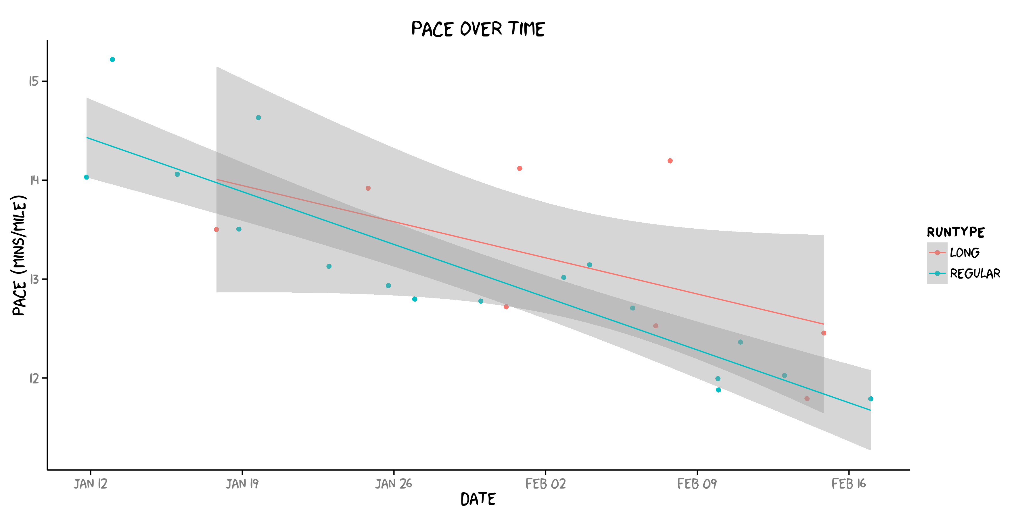
Here’s what my training runs look like. Look how slow I am!! Plotting xkcd style to emphasize both that I am not a runner and this is not real scientific analysis.
I’ve cut about 2′ off my pace in the last month, which means in 6 months, I’ll run a zero minute mile! (JOKE!! I’ll clearly go back to the future.) To be fair, I started running in snow and switched to a treadmill with this cold Chicago weather, so I don’t expect to keep improving this quickly. And I just got new shoes in the last week after being fit for them at a real running store because apparently I didn’t even know my actual shoe size, go figure. Also, I clearly started running at too slow a “cadence” (too few steps per minute, i.e., frequency) because I thought running faster meant I should increase my “stride” (i.e., wavelength). HA! That was clearly wrong. Running at 170-180 steps per minute was probably the best running advice I read.
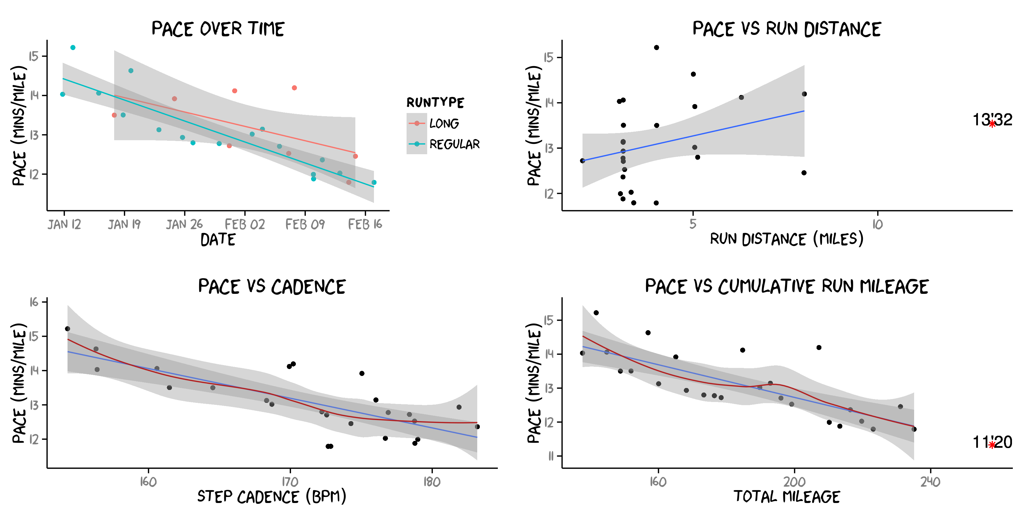
I made some projected guesstimates marked in the plots by red asterisks. The top right shows what I think a current comfortable half marathon pace for me would be given my current 5 weeks of training- meaning I think I could run a 13’32” pace half marathon this weekend basically. The bottom right plot shows (think this is probably the limit) how fast my average pace could be after another week of accumulating training mileage. So at the end of this week, I won’t expect to be any faster than about 11’20”. If you care about the details, just look at my code below. Also, I’m just using this to mess around with- you generally shouldn’t try and extrapolate far outside of your data (like this related ridiculousness: Projected sprint times for men vs women in the 2156 Olympics).
Anyway, glad to have some base code to help with my training. I’ll write another post with updated data and more runs around the half marathon.
library(RCurl)
library(rjson)
library(plyr)
library(scales)
library(ggplot2)
library(gridExtra)
library(extrafont)
library(xkcd)
#--------------------------------------------------------------------------
# INPUTS
accTokenFnm <- "accessToken.txt" # Put your api key in here
count <- 25 # number of runs to plot
#--------------------------------------------------------------------------
baseAddr <- "https://api.nike.com/"
header <- c(Accept="application/json", "Content-Type"="application/json", appid="fuelband")
#--------------------------------------------------------------------------
# Get user's access token
#--------------------------------------------------------------------------
getNikeAccessToken <- function(fnm=accTokenFnm){
accessTokenFile <- file(fnm, "rt", blocking=T)
accessToken <- readLines(accessTokenFile, 1, ok=T, warn=F)
close(accessTokenFile)
return(accessToken)
}
#--------------------------------------------------------------------------
# Get list of all activities
# Nike returns "data" and "paging". "data" contains url param "count" runs.
# Each run contains 9 values one of which is sublist
#--------------------------------------------------------------------------
listNikeRuns <- function(count, accessToken){
address <- paste(baseAddr, "me/sport/activities/", sep="")
num <- as.character(count*10) #getting 10 times more bc weird non-runs
url <- paste(address, "?access_token=", accessToken, "&count=", num, sep="")
json <- getURL(url, httpheader=header)
data <- fromJSON(json)
# Extract only interesting data for each run (returns list of list)
vars <- c("activityId", "startTime")
extracted <- lapply(data$data, function(d) d[vars])
# Now bind into df
df <- as.data.frame(t(sapply(extracted, function(x) rbind(x))))
names(df) <- names(extracted[[1]])
df <- df[- grep('-', df$activityId),] # getting rid of non-run weirdness
rownames(df) <- NULL
df$startTime <- gsub("T"," ", df$startTime)
df$startTime <- gsub("Z","", df$startTime)
df$startTime <- as.POSIXct(strptime(df$startTime, "%Y-%m-%d %H:%M:%S"))
return(head(df,count))
}
#--------------------------------------------------------------------------
# Download single run stats
# Nike returns some overall data.
#--------------------------------------------------------------------------
getNikeSingleRunStat <- function(activityId, accessToken){
message(paste("Downloading run", activityId, "..."))
address <- paste(baseAddr, "me/sport/activities/", sep="")
url <- paste(address, activityId, "?access_token=", accessToken, sep="")
json <- getURL(url, httpheader=header)
data <- fromJSON(json)
df <- as.data.frame(data$startTime)
df$activityId <- activityId
names(df) <- c('startTime','activityId')
df$startTime <- gsub("T"," ", df$startTime)
df$startTime <- gsub("Z","", df$startTime)
df$startTime <- as.POSIXct(strptime(df$startTime, "%Y-%m-%d %H:%M:%S"))
df$calories <- data$metricSummary$calories
df$fuel <- data$metricSummary$fuel
df$steps <- data$metricSummary$steps
df$distancekm <- data$metricSummary$distance
df$distancemi <- df$distancekm*.621371
df$duration <- data$metricSummary$duration
time <- as.numeric(strsplit(df$duration,':')[[1]])
df$totalmins <- time[1]*60 + time[2] + time[3]/60
df$avepace <- df$totalmins/df$distancemi
df$avepacemph <- df$distancemi /df$totalmins*60
df$cadence <- df$steps/df$totalmins
return(df)
}
#--------------------------------------------------------------------------
# Get actual data and make some plots
#--------------------------------------------------------------------------
accessToken <- getNikeAccessToken()
runs <- listNikeRuns(count, accessToken)
myrunlist <- list()
i <- 1
for (run in runs$activityId) {
myrunlist[[i]] <- getNikeSingleRunStat(run, accessToken)
i <- i+1
}
runStats <- Reduce(function(...)merge(...,all=T),myrunlist)
runStats$cumMileage <- cumsum(runStats$distancemi)
runStats$weekdays <- weekdays(runStats$startTime)
runStats$runtype[runStats$weekdays=='Saturday'] <- 'long' # all my Saturday runs are 'long' runs
runStats$runtype[runStats$weekdays!='Saturday'] <- 'regular'
runStats$runtype <- as.factor(runStats$runtype)
# avepace vs time
p1 <- ggplot(runStats, aes(x=startTime, y=avepace, colour=runtype)) + geom_point() +theme_xkcd() + theme(axis.line = element_line(colour = "black"))
p1 <- p1 + labs(x='Date', y='Pace (mins/mile)',title='Pace over time')
p1 <- p1 + geom_smooth(method='glm',se=TRUE)
# avepace vs run distance
p2 <- ggplot(runStats, aes(x=distancemi, y=avepace)) + geom_point() +theme_xkcd()+ theme(axis.line = element_line(colour = "black"))
p2 <- p2 + labs(x='Run distance (miles)', y='Pace (mins/mile)', title='Pace vs Run Distance')
p2 <- p2 + geom_smooth(method='glm',se=TRUE)
p2fit <- glm(avepace ~ distancemi + cadence + runtype, data=runStats)
# Predict pace by run distance and cadence
p2pred <- predict(p2fit, newdata= data.frame(distancemi=13.1,cadence=175, runtype='regular'))
p2 <- p2 + geom_point(aes(x=13.1,y=p2pred),color='red',shape=8)
p2 <- p2 + geom_text(aes(x=13.1,y=p2pred+.1), label=paste0(as.character(floor(p2pred)) , "'", as.character( round((round(p2pred,2)-floor(p2pred))*60),0 )))
# avepace vs cadence
p3 <- ggplot(runStats[runStats$cadence > 0,], aes(x=cadence, y=avepace)) + geom_point()+theme_xkcd()+ theme(axis.line = element_line(colour = "black"))
p3 <- p3 + labs(x='Step cadence (bpm)', y='Pace (mins/mile)', title='Pace vs Cadence')
p3 <- p3 + geom_smooth(method='glm',se=TRUE)
p3 <- p3 + stat_smooth(color='firebrick')
# avepace vs cumulative run mileage
p4 <- ggplot(runStats, aes(x=cumMileage, y=avepace)) + geom_point() +theme_xkcd()+ theme(axis.line = element_line(colour = "black"))
p4 <- p4 + labs(x='Total mileage', y='Pace (mins/mile)', title='Pace vs Cumulative Run Mileage')
p4 <- p4 + geom_smooth(method='glm',se=TRUE)
p4 <- p4 + stat_smooth(color='firebrick')
p4fit <- glm(avepace ~ cumMileage, data=runStats)
# Predict next week's pace by this week's expected cumulative mileage (not really good to extrapolate, but whatever)
p4pred <- predict(p4fit, newdata=data.frame(cumMileage=23+max(runStats$cumMileage)))
p4 <- p4 + geom_point(aes(x=23+max(runStats$cumMileage),y=p4pred),color='red',shape=8)
p4 <- p4 + geom_text(aes(x=23+max(runStats$cumMileage),y=p4pred+.1), label=paste0(as.character(floor(p4pred)) , "'", as.character( round((round(p4pred,2)-floor(p4pred))*60),0 )))
grid.arrange(p1,p2,p3,p4, nrow=2)
g <- arrangeGrob(p1,p2,p3,p4, nrow=2)Also, here’s my R sessionInfo() :
R version 3.1.1 (2014-07-10)
Platform: x86_64-pc-linux-gnu (64-bit)

locale:
 [1] LC_CTYPE=en_US.UTF-8       LC_NUMERIC=C
 [3] LC_TIME=en_US.UTF-8        LC_COLLATE=en_US.UTF-8
 [5] LC_MONETARY=en_US.UTF-8    LC_MESSAGES=en_US.UTF-8
 [7] LC_PAPER=en_US.UTF-8       LC_NAME=C
 [9] LC_ADDRESS=C               LC_TELEPHONE=C
[11] LC_MEASUREMENT=en_US.UTF-8 LC_IDENTIFICATION=C

attached base packages:
[1] grid      stats     graphics  grDevices utils     datasets  methods
[8] base

other attached packages:
[1] scales_0.2.4    plyr_1.8.1      rjson_0.2.15    RCurl_1.95-4.5
[5] bitops_1.0-6    xkcd_0.0.4      extrafont_0.17  gridExtra_0.9.1
[9] ggplot2_1.0.0

loaded via a namespace (and not attached):
 [1] acepack_1.3-3.3     cluster_1.15.3      colorspace_1.2-4
 [4] digest_0.6.4        extrafontdb_1.0     foreign_0.8-61
 [7] Formula_1.2-0       gtable_0.1.2        Hmisc_3.14-6
[10] labeling_0.3        lattice_0.20-29     latticeExtra_0.6-26
[13] MASS_7.3-35         munsell_0.4.2       nnet_7.3-8
[16] proto_0.3-10        RColorBrewer_1.0-5  Rcpp_0.11.3
[19] reshape2_1.4        rpart_4.1-8         Rttf2pt1_1.3.3
[22] splines_3.1.1       stringr_0.6.2       survival_2.37-7