Recently, I’ve been working on analysis of geospatial data. I found that there was a bit of a sharp learning curve just to be able to do some preliminary visualizations of spatial data, so this post will be a tutorial in some simple map visualizations with R. Note that this is really just useful for exploratory visual analysis.
I’ve been working with data over the entire US with data points for each county. You could do the same sort of thing as I am doing here if you have a list of data values with latitude and longitude coordinates or county (or state) FIPS codes.
For now, let’s just look at county populations. I’m going to map these data by the location of county population centroid (so by latitude and longitude coordinates, ie points). You could also look at the data by county polygons given by a shapefile (by FIPS code), but I’ll save choropleth mapping for another post.
First, I’m going to grab some public data on the county populations and locations of county population centroids in the US from the 2010 census.
fileUrl <- 'https://www.census.gov//geo/reference/docs/cenpop2010/county/CenPop2010_Mean_CO.txt'
download.file(fileUrl,destfile='CenPop2010_Mean_CO.txt',method='curl')
centroidsDF <- read.csv('CenPop2010_Mean_CO.txt',header=T,colClasses=c('character','character','character','character','integer','numeric','numeric'))
centroidsDF$fipscode <- as.integer(paste0(centroidsDF$STATEFP,centroidsDF$COUNTYFP))
Let’s look at the data.
head(centroidsDF)
## STATEFP COUNTYFP COUNAME STNAME POPULATION LATITUDE LONGITUDE fipscode
## 1 01 001 Autauga Alabama 54571 32.50 -86.49 1001
## 2 01 003 Baldwin Alabama 182265 30.55 -87.76 1003
## 3 01 005 Barbour Alabama 27457 31.84 -85.31 1005
## 4 01 007 Bibb Alabama 22915 33.03 -87.13 1007
## 5 01 009 Blount Alabama 57322 33.96 -86.59 1009
## 6 01 011 Bullock Alabama 10914 32.12 -85.70 1011</pre>
Restrict to the continental United States.
centroidsDF <- subset(centroidsDF, STATEFP!= "02") # alaska
centroidsDF <- subset(centroidsDF, STATEFP!= "15") # hawaii
centroidsDF <- subset(centroidsDF, STATEFP!= "72") # puerto rico
Now that I have a dataframe of latitude and longitude points, I’ll drop some columns and convert to a spatial object in R.
library(sp)
library(rgdal)
points <- as.data.frame(cbind(centroidsDF$LONGITUDE, centroidsDF$LATITUDE,centroidsDF$fipscode,centroidsDF$POPULATION))
names(points) <- c('lon','lat','fipscode','population')
### Turn into spatial object
coordinates(points) <- ~lon + lat
## Project for a nice display of county data across US
aea.proj <- "+proj=aea +lat_1=29.5 +lat_2=45.5 +lat_0=37.5 +lon_0=-102
              +x_0=180 +y_0=50 +ellps=GRS80 +datum=NAD83 +units=m"
proj4string(points) <- CRS("+proj=longlat")
points <- spTransform(points, CRS(aea.proj))
class(points)
## [1] "SpatialPointsDataFrame"
## attr(,"package")
## [1] "sp"
Now I have a SpatialPointsDataFrame object. Great! I’d like to plot it over a map of the US. So I’ll grab shapefile data also from the following link and unzip the contents into my working directory: http://www2.census.gov/geo/tiger/GENZ2010/gz_2010_us_050_00_5m.zip
I’ll manipulate this data a little bit to plot nicely.
### Read in US county shapefiles

all_counties <- readOGR("gz_2010_us_050_00_5m.shp", "gz_2010_us_050_00_5m")
## OGR data source with driver: ESRI Shapefile
## Source: "gz_2010_us_050_00_5m.shp", layer: "gz_2010_us_050_00_5m"
## with 3221 features and 6 fields
## Feature type: wkbPolygon with 2 dimensions

### Change projection of counties for nice plotting
all_counties <- spTransform(all_counties, CRS(aea.proj))
# Restrict to continental US for the moment
usa_counties <- subset(all_counties,STATE!= "02") #alaska
usa_counties <- subset(usa_counties,STATE!= "15") #hawaii
usa_counties <- subset(usa_counties,STATE!= "72") #puerto rico
class(usa_counties)
## [1] "SpatialPolygonsDataFrame"
## attr(,"package")
## [1] "sp"

 ### Create county borders
 county_borders <- as(usa_counties, "SpatialPolygonsDataFrame")
 ### Create state borders by combining counties
 library(maptools)
 library(gpclib)
 gpclibPermit()
 ## [1] TRUE
 state_borders <- unionSpatialPolygons(usa_counties, as.numeric(county_borders@data$STATE))</pre>
Make plots of the US population. I like to use ggplot2, since I think those plots look the nicest.
library(ggplot2)
methods(fortify)

## This plots an outline of counties.

countiesPlot <- ggplot(county_borders) + geom_polygon(aes(long,lat,group=group),fill=NA,col='black') + coord_equal()
 plot(countiesPlot)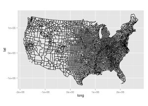
## This plots an outline of states.

statesPlot <- ggplot(state_borders) + geom_polygon(aes(long,lat,group=group),fill=NA,col='black') + coord_equal()
 plot(statesPlot)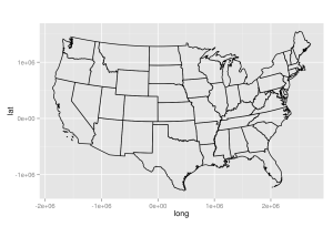
## Here is a plot of all the county population centroids alone.

pointsPlot <- ggplot(as(points,"data.frame")) + geom_point(aes(lon,lat,colour=population),alpha=0.5) + coord_equal() + scale_colour_gradient2(trans="log",guide=FALSE)
 plot(pointsPlot)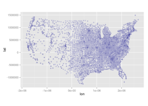
## This plots an outline of states and the population centroids on top, you could do the same for counties if you wanted to, but that seems like overkill to me.

statesPointsPlot <- statesPlot + geom_point(data = as(points,'data.frame'),aes(lon,lat,colour=population),alpha=0.5) + scale_colour_gradient2(trans="log",guide=FALSE)
plot(statesPointsPlot)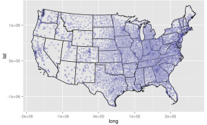
And that’s how you overlay a map of data values with latitude and longitude coordinates on a continental US map using R’s ggplot2. Happy mapping!!
## R version 3.1.1 (2014-07-10)
## Platform: x86_64-pc-linux-gnu (64-bit)
##
## locale:
##  [1] LC_CTYPE=en_US.UTF-8       LC_NUMERIC=C
##  [3] LC_TIME=en_US.UTF-8        LC_COLLATE=en_US.UTF-8
##  [5] LC_MONETARY=en_US.UTF-8    LC_MESSAGES=en_US.UTF-8
##  [7] LC_PAPER=en_US.UTF-8       LC_NAME=C
##  [9] LC_ADDRESS=C               LC_TELEPHONE=C
##
## attached base packages:
## [1] stats     graphics  grDevices utils     datasets  methods   base
##
## other attached packages:
## [1] sp_1.0-15     ggplot2_1.0.0
##
## loaded via a namespace (and not attached):
##  [1] colorspace_1.2-4 digest_0.6.4     evaluate_0.5.5   formatR_1.0
##  [5] grid_3.1.1       gtable_0.1.2     htmltools_0.2.6  knitr_1.6
##  [9] labeling_0.3     lattice_0.20-29  MASS_7.3-35      munsell_0.4.2
## [13] plyr_1.8.1       proto_0.3-10     Rcpp_0.11.3      reshape2_1.4
## [17] rmarkdown_0.3.3  scales_0.2.4     stringr_0.6.2    tools_3.1.1