One of the nice perks about working at a University is the opportunity to go to a wide variety of all kinds of classes and workshops. I just went to a really great workshop about Image Analysis in Python, given by Brian Keating, a UChicago RCC staff member. The materials for the class are on the lecturer’s Github:

https://github.com/brikeats/Image-Analysis-in-Python.

The post below is the code I wrote to count change in a picture Brian provided as a hands-on exercise. Please note that a blank copy of the guided steps (marked here in bold/italics), as well as another sample solution, are independently and originally available from Brian’s course materials- I’m just wanting to share here the code I filled in for each step (and heavily cribbed from the intro workshop materials).

This is the initial picture for analysis, containing only quarters, dimes and pennies (no nickels).

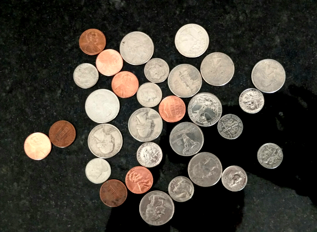
Step 1: Reading & displaying the image. Use matplotlib to read the file “sample-images/quarters_dimes_pennies.png”. Convert it to grayscale and display both the original and grayscale images.

import numpy as np
import matplotlib.pyplot as plt
from skimage import color
%matplotlib inline

def my_imshow(im, title=None, **kwargs):
    if 'cmap' not in kwargs:
        kwargs['cmap'] = 'gray'
    plt.figure()
    plt.imshow(im, interpolation='none', **kwargs)
    if title:
        plt.title(title)
    plt.axis('off')

im = plt.imread('sample-images/quarters_dimes_pennies.png')
gray_im = color.rgb2gray(im)

my_imshow(im)
my_imshow(gray_im)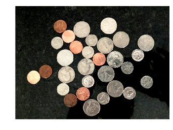

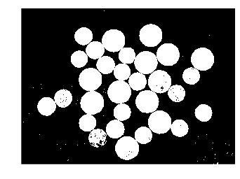
Step 2: Thresholding. Create a binary mask by thresholding the grayscale image. You can use a histogram and some guesswork to determine the threshold or use one of the threshold functions in skimage.filters. I’m using Ostu’s method.

from skimage.filters import threshold_otsu

thresh = threshold_otsu(gray_im, nbins=5)

thresholded = gray_im > thresh

plt.figure()
plt.hist(gray_im.ravel(), bins=100);
plt.plot([thresh, thresh], [0, 6000], linewidth=3, color='r');

my_imshow(thresholded)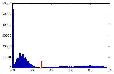

Step 3: Cleaning up the mask. Your mask will inevitably have some noise. Use morphology operators to clean up the mask. It doesn’t have to be 100% perfect, but you should be able to get rid of the specks.

from skimage import morphology
from skimage.morphology import disk

no_small = morphology.remove_small_objects(thresholded, min_size=150)

coins = morphology.binary_closing(no_small,disk(3))
plt.figure()
plt.imshow(coins, cmap='gray', interpolation='none')
plt.title('closed coins with small objects removed')
plt.axis('off')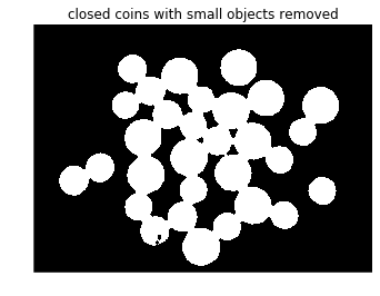

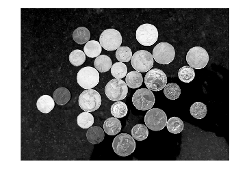
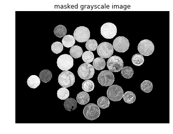
Step 4: Masking. It will be convenient to set the background to black. Use the coin mask that you created to set the backgrounds of both the original color image, and the grayscale image to zero. You should be able to see the coins in color, but the counter (and the reflections in the counter) should be black. While you’re at it, set the background of the grayscale image to zero as well. From now on, we don’t have to worry about the background affecting our results because we’ve masked it out.

im[coins==False] = 0
gray_im[coins==False] = 0


plt.figure()
plt.imshow(im, cmap='gray', interpolation='none')
plt.title('masked image')
plt.axis('off')

plt.figure()
plt.imshow(gray_im, cmap='gray', interpolation='none')
plt.title('masked grayscale image')
plt.axis('off')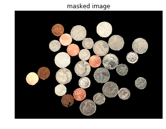

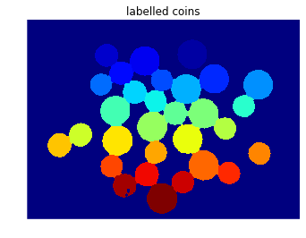
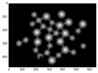
Step 5: Watershed Segmentation Now that we’ve segmented the foreground from the background, we want to distinguish the coins from each other. Use the watershed-based segmentation that was introduced in the cell counting demo to create a label image for the coins. Print the number of coins in the image.

from scipy import ndimage as ndi
from matplotlib.colors import ListedColormap

distance_im = ndi.distance_transform_edt(coins)
print 'distance transform:', distance_im.shape, distance_im.dtype

from skimage import feature, measure

def imshow_overlay(im, mask, alpha=0.5, color='red', **kwargs):
    """Show semi-transparent red mask over an image"""
    mask = mask > 0
    mask = np.ma.masked_where(~mask, mask)        
    plt.imshow(im, **kwargs)
    plt.imshow(mask, alpha=alpha, cmap=ListedColormap([color]))


peaks_im = feature.peak_local_max(distance_im, indices=False)

plt.figure()
imshow_overlay(distance_im, peaks_im, alpha=1, cmap='gray')

markers_im = measure.label(peaks_im)
labelled_coins = morphology.watershed(-distance_im, markers_im, mask=coins)
num_coins = len(np.unique(labelled_coins))-1  # subtract 1 b/c background is labelled 0
print 'number of coins: %i' % num_coins

my_imshow(labelled_coins, 'labelled coins', cmap='jet')

distance transform: (475, 649) float64
number of coins: 30

Step 6: Quantifying & displaying the object sizes. Look up the documentation for scikit-image function regionprops online. Use this function with the labelled coins image to compute the area of each coin and the location of each coin’s center (the center is called the “centroid”). Display the image and use matplotlib’s text function to write the area of each coin at its center.

my_imshow(im, 'labelled coins', cmap='jet')

properties = measure.regionprops(labelled_coins)
coin_areas = [int(prop.area) for prop in properties]
coin_centroids = [prop.centroid for prop in properties]

for lab in range(len(coin_areas)):
    plt.text(coin_centroids[lab][1]-30,coin_centroids[lab][0],coin_areas[lab])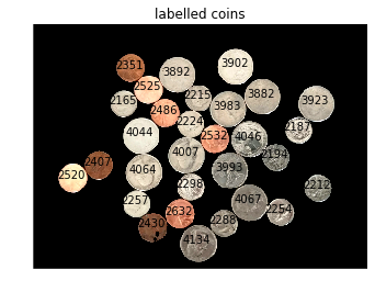

Step 7: Separate coins by size & count. It is possible to sort the coins on the basis of size. By trial and error, select size thresholds that can use a region’s area to determine the coin’s denomination. Count the number of each denomination, and print the total value of the coins in the image.

properties = measure.regionprops(labelled_coins)

coin_areas = np.array([prop.area for prop in properties])

print coin_areas

plt.figure()
plt.hist(coin_areas, bins=10)
plt.show()
plt.axis('off')

#print num_each_coin
num_dimes = len(np.where(coin_areas < 2300)[0])
num_pennies = len(np.where( (2300 < coin_areas) & (coin_areas < 3500))[0])
num_quarters = len(np.where(coin_areas > 3500)[0])

print 'number of dimes: %i' % num_dimes
print 'number of pennies: %i' % num_pennies
print 'number of quarters: %i' % num_quarters
print 'Total value in image: $%.2f' % (num_dimes*.10 + num_pennies*.01 + num_quarters*.25)

[ 3902.  2351.  3892.  2525.  3882.  2215.  2165.  3923.  3983.  2486.
  2224.  2187.  4044.  2532.  4046.  4007.  2194.  2407.  3993.  4064.
  2520.  2298.  2212.  4067.  2257.  2254.  2632.  2288.  2430.  4134.]

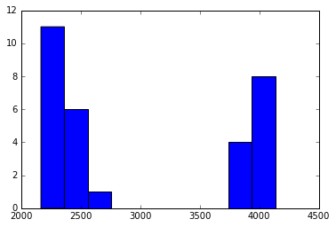
number of dimes: 10
number of pennies: 8
number of quarters: 12
Total value in image: $4.08

So $4.08 in the image! Looks about right. The thresholding on coin sizes at the end could be improved by perhaps either using colors of the coins or by doing some sort of clustering algorithm on the regions, knowing that there are only 3 types of coins. Good start anyway and a really great hands-on workshop exercise.